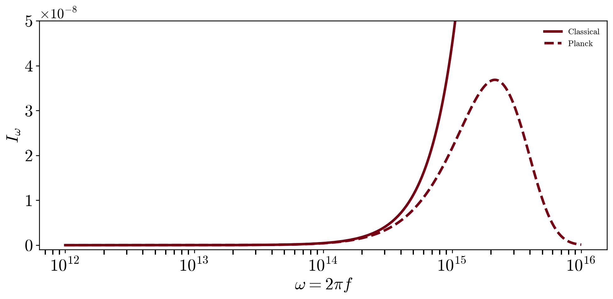
The classical black-body spectrum was
import matplotlib.pyplot as plt
import numpy as np
# plotstyle re-exports plottools with the site's 'blog_post' figure style
# already selected, so no style= argument is needed at any call site below.
import plotstyle as pt

# Constants
h = 6.63e-34            # J*s
k = 1.38e-23            # J/K
c = 3e8                 # m/s
def wavelength(omega):
    return 2*np.pi / omega

# Radiation spectra
def rayleigh_jeans(T, scale=1):
    def f(omega):
        nu = omega / (2*np.pi)
        return scale * 2*(nu**2)*k*T/(c**2)
    return f
def planck_law(T, scale=1):
    def f(omega):
        nu = omega / (2*np.pi)
        return scale * 2*h*(nu**3)/(c**2) / (np.exp(h*nu/(k*T)) - 1)
    return f
T = 5800            # temp of sun in Kelvin
rj = rayleigh_jeans(T)
planck = planck_law(T)

# Plot the spectra
T_rng = [1e12, 1e16]
fig, axes = pt.add_subplots(); ax = axes[0]
pt.plot_1d_func(rj, ax = ax, x_bounds = T_rng, nx = 500, ax_label = [r'$\omega=2\pi f$', r'$I_\omega$'], fn_label = 'Classical')
pt.plot_1d_func(planck, ax = ax, x_bounds = T_rng, nx = 500, ls = '--', ax_label = [r'$\omega=2\pi f$', r'$I_\omega$'], fn_label = 'Planck')
ax.set_xscale('log')
ax.set_ylim((-1e-9, 5e-8))
ax.legend(framealpha = 0)
The figure above was generated when this page was rendered, not pasted in.